Negative Binomial Regression

When counts vary more than Poisson allows

About this page: an AI-first draft

Like the Ordinal Regression page, this was drafted first by an AI assistant (Claude Fable) and is offered as a starting point for me to revise. It is part of closing a gap that opened when the GLM Dashboard Explainer ran ahead of these notes: the dashboard has a full negative-binomial tutorial, while JonStats had nothing on overdispersion at all. The R code is real and runnable; the prose deserves a careful read.

Where this fits

The organising idea of these notes is the two-part model (after King, Tomz & Wittenberg, 2000): a stochastic component for what kind of random thing the response is, and a systematic component for how the predictors move it.

Y_i \sim f(\theta_i, \alpha) \qquad\qquad \theta_i = g(X_i, \beta)

Poisson regression is the standard first model for counts: f is the Poisson distribution and g is the log link. But Poisson comes with a hidden promise that real count data routinely breaks. Negative binomial regression keeps the same systematic side and the same log link — it only changes f, and in doing so it puts the usually-ignored parameter \alpha to work.

flowchart LR
  X
  beta
  eta
  f
  alpha
  Y
  X --> eta
  beta --> eta
  eta --> f
  alpha --> f
  f --> Y

Everything on this page is about that \alpha — the dispersion — flowing into f.

The data: counts that won’t sit still

We’ll use MASS::quine: the number of days each of 146 Australian schoolchildren was absent in a year, with predictors for ethnicity, sex, age group and learning ability.

Code

library(MASS)
data(quine)
c(mean = mean(quine$Days), variance = var(quine$Days))

    mean variance 
 16.4589 264.1673

The variance is roughly sixteen times the mean. That single fact is the whole problem, because of a peculiarity of the Poisson distribution.

Why Poisson isn’t enough

The Poisson distribution has exactly one parameter, and it does double duty: the mean and the variance are the same number,

\operatorname{Var}(Y) = \operatorname{E}(Y) = \mu.

That is a strong, testable claim — and counts in the wild rarely honour it. Real count data are usually overdispersed: more variable than their mean, because of unmeasured heterogeneity (some children are simply more absence-prone than their predictors reveal).

We can see the strain directly. If the Poisson model were adequate, its residual deviance should be roughly equal to its residual degrees of freedom:

Code

m_pois <- glm(Days ~ Eth + Sex + Age + Lrn, family = poisson, data = quine)
c(resid_deviance = deviance(m_pois),
  df             = df.residual(m_pois),
  ratio          = deviance(m_pois) / df.residual(m_pois))

resid_deviance             df          ratio 
    1696.70655      139.00000       12.20652

A ratio near twelve, where we wanted one, is the model telling us it cannot account for how spread out the data are. The coefficients may not be badly wrong, but the uncertainty the model reports will be — far too small, as we’ll see.

The negative binomial fix

The negative binomial keeps the mean model \mu_i = \exp(X_i\beta) untouched and adds a single dispersion parameter \theta that lets the variance grow faster than the mean:

\operatorname{Var}(Y) = \mu + \frac{\mu^2}{\theta}.

This is a variance function — a statement about how spread depends on level — and it is the first time in this course that the “uninteresting” stochastic parameter \alpha has become the point of the exercise. As \theta \to \infty the extra term vanishes and the negative binomial collapses back to the Poisson; small \theta means heavy overdispersion. Picturing the two variance functions side by side makes the difference concrete:

Code

library(ggplot2)
m_nb  <- glm.nb(Days ~ Eth + Sex + Age + Lrn, data = quine)
theta <- m_nb$theta
mu    <- seq(0, 60, length.out = 200)

vf <- rbind(
  data.frame(mu = mu, variance = mu,                  model = "Poisson:  Var = mu"),
  data.frame(mu = mu, variance = mu + mu^2 / theta,   model = "Negative binomial:  Var = mu + mu^2 / theta")
)

ggplot(vf, aes(mu, variance, colour = model)) +
  geom_line(linewidth = 1) +
  labs(x = "mean count (mu)", y = "variance", colour = NULL,
       title = "Two variance functions") +
  theme_minimal() +
  theme(legend.position = "top")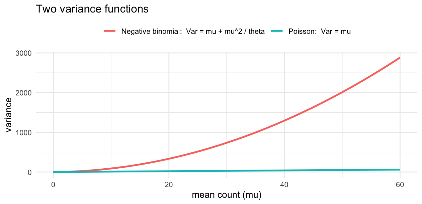

Poisson forces the variance to equal the mean (the straight line). The negative binomial lets it curve upward, with the fitted dispersion theta controlling how sharply.

Fitting it in R

MASS::glm.nb fits the negative binomial, estimating \theta alongside the coefficients:

Code

summary(m_nb)


Call:
glm.nb(formula = Days ~ Eth + Sex + Age + Lrn, data = quine, 
    init.theta = 1.274892646, link = log)

Coefficients:
            Estimate Std. Error z value Pr(>|z|)    
(Intercept)  2.89458    0.22842  12.672  < 2e-16 ***
EthN        -0.56937    0.15333  -3.713 0.000205 ***
SexM         0.08232    0.15992   0.515 0.606710    
AgeF1       -0.44843    0.23975  -1.870 0.061425 .  
AgeF2        0.08808    0.23619   0.373 0.709211    
AgeF3        0.35690    0.24832   1.437 0.150651    
LrnSL        0.29211    0.18647   1.566 0.117236    
---
Signif. codes:  0 '***' 0.001 '**' 0.01 '*' 0.05 '.' 0.1 ' ' 1

(Dispersion parameter for Negative Binomial(1.2749) family taken to be 1)

    Null deviance: 195.29  on 145  degrees of freedom
Residual deviance: 167.95  on 139  degrees of freedom
AIC: 1109.2

Number of Fisher Scoring iterations: 1

              Theta:  1.275 
          Std. Err.:  0.161 

 2 x log-likelihood:  -1093.151

The coefficient block reads exactly like a Poisson fit — same log link, same kind of log-rate coefficients. What is new is the line beneath it reporting the estimated dispersion:

Code

m_nb$theta

[1] 1.274893

A small \theta like this confirms heavy overdispersion. And the model comparison is decisive — the negative binomial is an enormously better fit for the same predictors:

Code

AIC(m_pois, m_nb)

       df      AIC
m_pois  7 2299.184
m_nb    8 1109.151

Why only betas look at betas (again)

A recurring lesson in these notes is that the raw coefficients are seldom the thing to read off directly. With a log link they are log rate ratios, so the interpretable quantity is their exponential:

Code

round(exp(coef(m_nb)), 3)

(Intercept)        EthN        SexM       AgeF1       AgeF2       AgeF3 
     18.076       0.566       1.086       0.639       1.092       1.429 
      LrnSL 
      1.339

Each value multiplies the expected count. So switching the Eth indicator multiplies the expected number of absences by about 0.57 (roughly a 43% reduction), holding the other predictors fixed.

But the deeper lesson here is about the numbers you didn’t ask to see — the standard errors. The Poisson and negative binomial models give nearly the same point estimates, yet very different standard errors, because the Poisson model wrongly believes the data are far tidier than they are. Fitting Poisson to overdispersed counts produces standard errors that are too small, t-statistics that are too large, and a procession of significance stars that should not be there. This is the count-data face of the warning in the P-Values and Statistical Significance notes: a model that misstates the variance will misstate your confidence, and overdispersion is one of the commonest ways for that to happen quietly.

Quasi-Poisson and other routes

The negative binomial is not the only response to overdispersion.

Quasi-Poisson (family = quasipoisson) takes a blunter approach: it keeps the Poisson mean model but multiplies all the standard errors by an estimated dispersion factor. It fixes the inference without committing to a full distribution for the counts — useful, but it cannot be compared by AIC because it has no likelihood.
Zero-inflation is a different problem again — an excess of zeros over what any single count distribution predicts, handled by a two-part mixture. The dashboard covers it as a separate tutorial; it stretches the framework further than this page does.

Try it interactively

The companion GLM Dashboard Explainer has an interactive negative-binomial walkthrough that lets you watch overdispersion break a Poisson fit and then be absorbed by the dispersion parameter: Tutorial 4: Overdispersed Counts.

Where this fits

The data: counts that won’t sit still

Why Poisson isn’t enough

The negative binomial fix

Fitting it in R

Why only betas look at betas (again)

Quasi-Poisson and other routes

Try it interactively

Further reading and connections