Beta Regression

When the response is a proportion

NoteAbout this page: an AI-first draft

As with the Ordinal and Negative Binomial pages, this was drafted first by an AI assistant (Claude Fable), to close a gap the GLM Dashboard Explainer had opened by running ahead of these notes. The R here is deliberately built from base R — we simulate data and fit it by hand — both so the page renders without extra packages and because that approach suits the likelihood-and-simulation spirit of this course. Read the prose critically before relying on it.

Where this fits

These notes keep returning to the two-part model (after King, Tomz & Wittenberg, 2000):

Y_i \sim f(\theta_i, \alpha) \qquad\qquad \theta_i = g(X_i, \beta)

Each model so far has been a particular choice of family f and link g. Beta regression is the choice for a response that is a continuous proportion — a number strictly between 0 and 1 — and it makes a point worth pausing on: it reuses the exact same logit link as logistic regression, but pairs it with a different distribution. Link and family are separate choices, and this is the cleanest demonstration of that in the whole course.

The data: proportions, rates and shares

Plenty of responses live on the open interval (0, 1) without being yes/no outcomes: the proportion of exam questions a student gets right, a candidate’s share of the vote in a constituency, the fraction of an insurer’s premiums paid out in claims, the proportion of a budget spent. These are continuous, but bounded.

Two familiar models both misfit them:

• Ordinary linear regression treats the response as unbounded, so it will cheerfully predict a proportion of 1.3 or -0.2, and it assumes a constant variance that a bounded quantity cannot have (a proportion near 0 or 1 simply has less room to vary).
• Logistic regression is for binary outcomes — counts of successes out of trials — not a continuous proportion that was never a count in the first place. Forcing a 0.73 to be “0.73 of a success” throws away the fact that it is a genuine measured fraction.

Beta regression keeps the response on (0,1) and lets its variance shrink toward the boundaries, where bounded data really do vary less.

The beta distribution

The beta distribution lives on (0, 1) and is usually written with two shape parameters, but for regression it is far more natural to reparameterise it in terms of a mean \mu and a precision \phi:

\operatorname{E}(Y) = \mu, \qquad \operatorname{Var}(Y) = \frac{\mu(1-\mu)}{1 + \phi}.

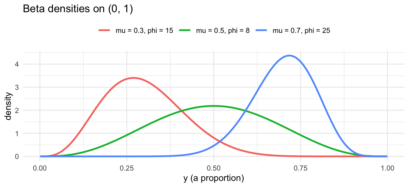
The mean \mu is what the predictors will steer; \phi plays the role that \sigma^2 does for the Gaussian or \theta does for the negative binomial — a dispersion-style parameter that the data also have to estimate. Larger \phi means more precise, i.e. less variance around the mean. The distribution’s great virtue is flexibility of shape while staying inside the boundaries:

library(ggplot2)

shapes <- list("mu = 0.3, phi = 15" = c(0.3, 15),
               "mu = 0.5, phi = 8"  = c(0.5, 8),
               "mu = 0.7, phi = 25" = c(0.7, 25))
grid <- do.call(rbind, lapply(names(shapes), function(nm) {
  p <- shapes[[nm]]
  x <- seq(0.001, 0.999, length.out = 300)
  data.frame(x = x, density = dbeta(x, p[1] * p[2], (1 - p[1]) * p[2]), shape = nm)
}))

ggplot(grid, aes(x, density, colour = shape)) +
  geom_line(linewidth = 1) +
  labs(x = "y (a proportion)", y = "density", colour = NULL,
       title = "Beta densities on (0, 1)") +
  theme_minimal() +
  theme(legend.position = "top")

The beta distribution takes many shapes on (0,1) — here for three (mean, precision) pairs — but never strays outside the boundaries, unlike a Gaussian.

The same logit link, a different distribution

To connect the mean to predictors we need a link that keeps \mu inside (0,1). That is exactly the job the logit did for logistic regression, and we use it again unchanged:

\mu_i = \operatorname{logit}^{-1}(X_i\beta) = \frac{1}{1 + e^{-X_i\beta}}.

So the logit keeps reappearing across this course, each time bolted onto a different family: binomial for binary outcomes (logistic regression, in Intro to GLMs); the cumulative form for ordered categories (Ordinal Regression); and now beta for continuous proportions. The link handles the constraint; the family handles the shape of the randomness. They are genuinely independent dials.

Fitting it: simulate, then recover

Beta regression in R is usually done with the betareg package, which is not part of base R. Rather than depend on it, we can lean on the likelihood and simulation theory developed earlier and do the whole thing from scratch: invent data with a known answer, then let an optimiser climb the log-likelihood back to it. If the machinery is sound, the estimates should land on the truth.

First, simulate proportions from a beta model with coefficients we choose:

set.seed(2024)
n  <- 300
x1 <- runif(n, -2, 2)
x2 <- rbinom(n, 1, 0.5)
X  <- cbind(1, x1, x2)

beta_true <- c(0.4, 0.8, -0.5)                 # intercept, x1, x2
phi_true  <- 15                                # precision
mu <- plogis(X %*% beta_true)                  # the logit link
y  <- rbeta(n, mu * phi_true, (1 - mu) * phi_true)

The beta log-likelihood for one observation, in the mean–precision parameterisation, is

\ell_i = \ln\Gamma(\phi) - \ln\Gamma(\mu_i\phi) - \ln\Gamma\!\big((1-\mu_i)\phi\big) + (\mu_i\phi - 1)\ln y_i + \big((1-\mu_i)\phi - 1\big)\ln(1-y_i),

which dbeta(..., log = TRUE) computes for us. We hand the negative of its sum to optim — the “Robo-Chauffeur” of the likelihood page — optimising \log\phi so the precision stays positive:

neg_loglik <- function(par) {
  beta <- par[1:3]
  phi  <- exp(par[4])                          # keep precision positive
  mu   <- plogis(X %*% beta)
  -sum(dbeta(y, mu * phi, (1 - mu) * phi, log = TRUE))
}

fit <- optim(c(0, 0, 0, 0), neg_loglik, method = "BFGS", hessian = TRUE)
se  <- sqrt(diag(solve(fit$hessian)))          # SEs from the Hessian, as on the likelihood page

data.frame(
  parameter = c("(Intercept)", "x1", "x2"),
  true      = beta_true,
  estimate  = round(fit$par[1:3], 3),
  std_error = round(se[1:3], 3)
)

    parameter true estimate std_error
1 (Intercept)  0.4    0.421     0.051
2          x1  0.8    0.807     0.030
3          x2 -0.5   -0.509     0.067

The estimates sit right on top of the true values, and the precision is recovered too:

c(true = phi_true, estimate = round(exp(fit$par[4]), 2))

    true estimate 
   15.00    13.72 

Note the standard errors came straight from the curvature of the log-likelihood at its peak — the inverse Hessian — exactly the connection between curvature and uncertainty made in the likelihood and simulation theory notes. The same Hessian an optimiser uses to find the peak efficiently is the one that tells you how sure to be once you are there.

The one-liner in practice

In day-to-day work nobody hand-rolls the likelihood; the betareg package wraps all of the above — and adds proper inference, a model for the precision, diagnostics and predictions — into a single call that mirrors glm:

library(betareg)
m <- betareg(y ~ x1 + x2)        # same estimates as above, plus full inference
summary(m)

That betareg is a separate package, rather than another family inside base R’s glm(), is itself instructive: the GLM framework reaches comfortably past the handful of families R ships with.

Why only betas look at betas (again)

Because the link is the logit, the coefficients are once more on the log-odds scale, not the proportion scale — so, as with logistic and ordinal regression, you cannot read a \beta off and call it an effect on the proportion. Map it through the inverse logit for a concrete profile, or read \exp(\beta) as an odds ratio, but do not stare at the raw number.

And the precision parameter \phi is worth a glance of its own. It is the beta family’s version of the negative binomial’s \theta and the Gaussian’s \sigma^2: a second, stochastic-side parameter that the data must estimate and that governs how tightly the responses cluster around the fitted mean. Across these extended families, the same lesson keeps surfacing — the \alpha in f(\theta, \alpha) is not always a nuisance to be ignored.

Try it interactively

TipTry it interactively

The companion GLM Dashboard Explainer has an interactive beta walkthrough — choosing a bounded-proportion response, seeing the logit link reused, and watching the beta distribution’s shape flex inside (0,1): Tutorial 6: Bounded Proportions.

Further reading and connections

• The link, reused. Intro to GLMs introduces the logit for logistic regression, and Ordinal Regression reuses it in cumulative form — beta regression is the third appearance of the same link.
• The machinery. Likelihood and Simulation Theory is where optim, the log-likelihood and the Hessian-as-uncertainty come from, and the Complete Simulation Example is the simulate-then-recover loop used above, in full.
• The interactive companion. The other extended families have tutorials on the GLM Dashboard Explainer.